Program description

Introduction

indexf is a program written in C++ to measure line-strength indices in fully calibrated FITS spectra. By fully calibrated one should understand wavelength and relative flux-calibrated data. Note that the different types of line-strength indices that can be measured with indexf (see below) do not require absolute flux calibration. If even a relative flux-calibration is absent (or deficient), the derived indices should be transformed to an appropriate spectrophotometric system.

The author thanks Sergio Pascual for his invaluable help to facilitate the installation procedure with autotools, as well as the maintenance of the source repository.

Error estimation

The program can also compute index errors resulting from the propagation of random errors (e.g. photon statistics, read-out noise). This option is only available if the user provides the error spectrum as an additional input FITS file to indexf. The error spectrum must contain the unbiased standard deviation (and not the variance!) for each pixel of the data spectrum. Full details of the formulae employed for the computation of errors in molecular and atomic indices, as well as in the D4000-like indices, are given in [Cardiel+98] and in chapter 2 of Cardiel’s thesis —in Spanish—; for the generic indices see Appendix A in [Cenarro+01b]. For a discussion on the impact of random errors in line-strength indices when studying stellar populations see [Cardiel+03].

In addition, indexf also estimates the effect of errors on radial velocity. For this purpose, the program performs Monte Carlo simulations by measuring each index using randomly drawn radial velocities (following a Gaussian distribution of a given standard deviation).

If no error file is employed, the program can perform numerical simulations with synthetic error spectra, the latter generated from the original data spectra and assuming randomly generated S/N ratios.

Index definitions

The line-strength indices that can be measured with indexf are those defined in the file indexdef.dat, located in the auxdir/ subdirectory of the distribution source code. The first column in this file is the identification name of each index (maximum 8 characters), as recognized by indexf. The second column, labeled as code, is an integer number that allows the identification of the type of line-strength feature. The code used in this column is the following:

index code	type of index	examples
1	molecular	CN1, CN2, Mg1, Mg2, TiO1, TiO2,…
2	atomic	Ca4227, G4300, Fe4668, Hbeta, Fe5270, Fe5335,…
3	D4000-like	D4000
4	B4000-like	B4000
5	Color-like	infrared CO_KH
10	Emission line	OII3727e
[11..99]	Generic discontinuity	D_CO,…
[101..9999]	Generic index	CaT, PaT, CaT*,…
[-99..-2]	Slope index	sTiO

Warning

Wavelengths in indexdef.dat in most indices are given in the air (except for those in the near-IR, like the D_CO; note however that the near-IR indices defined by [Eftekhari+21] are given in the air). If your spectra have been reduced using a wavelength calibration in vacuum, you can handle this by setting the parameter vacuum to 1, 2 or 3 when running the program (for the D_CO index you do not need to introduce a vacuum correction). See the use of vacuum in section Using the program for details.

An example of some of the definitions that can be found in the file indexdef.dat is the following (the list shown here is not complete!):

Index    code    blue bandpass      central bandpass      red bandpass     >              source
======== ====  ==================  ==================  ==================    ======================================
CN1         1  4080.125  4117.625  4142.125  4177.125  4244.125  4284.125  > Lick
HdA         2  4041.600  4079.750  4083.500  4122.250  4128.500  4161.000  > Hdelta A (Worthey & Ottaviani 1997)
D4000       3  3750.000  3950.000  4050.000  4250.000     0.000     0.000  > 4000 break (Bruzual 1983)
B4000       4  3750.000  3950.000  4050.000  4250.000     0.000     0.000  > 4000 break (Gorgas et al. 1999)
CO_KH       5  22872.83  22925.26  22930.52  22983.22  00000.00  00000.00  > Kleinmann & Hall (1986)
OII3727e   10  > emission line OII 3727
                4
                3660.000  3666.000  0.0
                3680.000  3688.000  0.0
                3710.000  3735.000  1.0
                3740.000  3750.000  0.0
D_CO       12  > generic CO discontinuity (Marmol-Queralto et al. 2008)
                22880.00  23010.00
                22460.00  22550.00
                22710.00  22770.00
CaT_star  506  > CaT* index from Cenarro et al.(2001) (Paschen-corrected near-IR Ca triplet)
                8474.000  8484.000
                8563.000  8577.000
                8619.000  8642.000
                8700.000  8725.000
                8776.000  8792.000
                8461.000  8474.000  -0.93
                8484.000  8513.000  1.0
                8522.000  8562.000  1.0
                8577.000  8619.000  -0.93
                8642.000  8682.000  1.0
                8730.000  8772.000  -0.93
sTiO       -5  > Near-IR spectral slope (Cenarro et al. in preparation)
                8474.000  8484.000
                8563.000  8577.000
                8619.000  8642.000
                8700.000  8725.000
                8776.000  8792.000

The two classical line-strength indices typically employed in the literature, molecular (index code = 1) and atomic (index code = 2) are defined with the help of 3 bandpasses, which appear in the following columns of each index entry of the file indexdef.dat. Among the most common sets of molecular and atomic indices, one of the most widely used is the Lick/IDS system (see e.g. [Trager+98] and references therein).
Two types of simple discontinuity indices are exemplified by the D4000 (index code = 3) and the B4000 (index code =4); see e.g. [Gorgas+99]. In both cases, the line-strength index is defined as the ratio between the integrated flux in two nearby bandpasses. The difference between the D4000 and the B4000 like indices is the way in which the flux in each bandpass is integrated. In D4000-like indices, and due to historical reasons (e.g. [Bruzual83]), the total flux in each bandpass is computed as the integral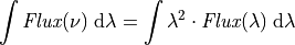

$\int{\mathit{Flux}(\nu)\; \mbox{d}\lambda} = \int{\lambda^2 \cdot \mathit{Flux(\lambda)} \; \mbox{d}\lambda}$

extended over the wavelength range of the considered bandpass.

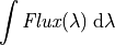
On the other hand, the total flux in each band of the B4000-like indices are obtained through the, more intuitive, integral of

$\int{\mathit{Flux(\lambda)} \; \mbox{d}\lambda}$
The color-like index (index code = 5), defined with two bandpasses as $-2.5\log_{10}[\mathit{Flux_{\rm blue}/Flux_{\rm red}}]$ , is exemplified by the CO index at 2.1 microns CO_KH (e.g. [KleinmannHall86]).
Emission line features (index code = 10) are measured by defining an arbitrary number of continuum and feature regions. The format to define this kind of index in the file indexdef.dat consists in providing the total number of regions in the second line, and the wavelength limits of each band followed by a factor in the subsequent lines. When this factor is equal to 0.0, the region is used to compute the continuum, whereas a factor equal to 1.0 indicates emission-line region (see e.g. definition of OII3727e). All the continuum regions are fitted using a straight line fit.
Generic discontinuities (index code: 11 ≤ n ≤ 99) can be used to define discontinuities with a variable number of wavelength regions at both sides of the discontinuity. The integer value of code in the second column of the file indexdef.dat is computed as

$\mathit{code} = \mathit{NC} \times 10 + \mathit{NA}$

where $\mathit{NC}$ and $\mathit{NA}$ are, respectively, the number of continuum and absorption spectral bandpasses at both sides of the discontinuity. For this kind of index, the wavelengths which define each bandpass are given in different rows in the file indexdef.dat For illustration, see [MarmolQueralto+08] for a detailed definition of the D_C0 index.
The generic indices constitute a generalization of the atomic indices, with the possibility of using an arbitrary number of continuum and spectral-feature bandpasses, being the contribution of the latter weigthed by arbitrary factors. This new type of index has been introduced in the empirical calibration of the near-IR Ca triplet (see details in [Cenarro+01b]). The integer value of “code” in the second column of the file indexdef.dat is computed as

$\mathit{code} = \mathit{NC} \times 100 + \mathit{NF}$

where $\mathit{NC}$ and $\mathit{NF}$ are, respectively, the number of continuum and spectral-feature bandpasses. For this kind of index, the wavelengths which define each bandpass are given in different rows in the file indexdef.dat, with the continuum bandpasses first. Note that the rows defining the spectral-feature bandpasses also contain, as a third column, the corresponding coefficient that should be applied to each of these bandpasses.
The slope indices are derived through the fit of a straight line to an arbitrary number of bandpasses (ranging from 2 to 99). The integer value of code in indexdef.dat indicates the number of bandpasses with a negative sign. The derived indices correspond to the ratio of two fluxes, evaluated at the central wavelength of the reddest and bluest bandpasses.

Although the file indexdef.da*t can be easily edited and modified by any program user to include new index definitions (of the type previously described), it is important to keep the file format in order to guarantee that **indexf* works properly. In order to facilitate this edition, since version 4.1.2 indexf looks first for a file called myindexdef.dat in the current (working) directory. If this file exists, the original indexdef.dat is ignored. So, I recommend the user to create a copy of the original indexdef.dat as myindexdef.dat in the working directory, and to modify the latter when necessary.